1 Introduction
Variational quantum algorithms (VQAs) optimise the parameters of a quantum circuit to minimise a cost . McClean et al. [1] showed that for circuits that are random enough to form unitary 2-designs, the gradient of has mean zero and a variance that shrinks exponentially with the number of qubits — a barren plateau (BP). A large literature has since characterised when plateaus occur: they depend on the locality of the cost [2], on the entanglement of the states the ansatz produces [3], on how parameters are initialised [4, 5], and, most generally, on the dimension of the dynamical Lie algebra (DLA) generated by the circuit [6, 7, 8]; see [9] for a review.
These results are precise and quantitative, and most of them can be tested on – qubits with a few hundred thousand cheap gradient evaluations. This report does exactly that, with two goals. The first is pedagogical and engineering-oriented: a transparent simulator with exact analytic gradients that fits in a few hundred lines, is verified against independent references and against an established library, and runs every experiment reported here on a single CPU core in under an hour. The second is scientific: to put the main theoretical predictions side by side with controlled numerics and to report the quantitative discrepancies and non-obvious behaviours that appear in the process.
Contributions.
Simulator. A NumPy state-vector simulator (
qsim) with in-place gate application, fast paths for diagonal and controlled gates, parameter-shift and adjoint-mode gradients supporting shared and scaled parameters (Sec. 3). It is 2–8 faster than PennyLane’sdefault.qubitfor the circuits used here, and returns the full gradient of 320 parameters at in s.Closed-form references. Haar-average gradient variances for a rotation with a 2-design before, after, or on both sides (Appendix A), verified numerically (Table 5).
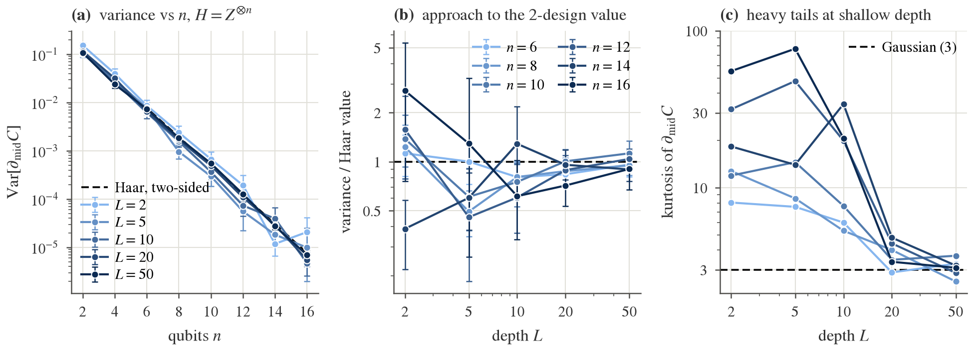
Approach to the plateau. The variance of a hardware-efficient ansatz converges to the two-sided Haar value non-monotonically with depth; the gradient distribution is heavy-tailed until it does; and the variance saturates long before the output entanglement does (Secs. 5.1–5.2).
Reproductions with quantified discrepancies. Cost locality (Sec. 5.3), initialisation strategies (Sec. 5.4), QAOA (Sec. 5.6).
Plateaus versus optimisation. With exact gradients Adam is insensitive to the plateau at these sizes; with realistic shot noise it is not (Sec. 5.5).
Lie-algebraic check. Exact DLA dimensions and -purities for four ansatz families, compared with the variance of deep circuits (Sec. 5.7).
2 Background and conventions
A parameterised circuit is a product of fixed gates and rotations with Hermitian, involutory generators (: Pauli strings). The angle is either fixed or , so that one parameter may drive several gates (as in QAOA) with a scale . Qubit is the most significant bit and rotations follow the convention of PennyLane and Qiskit. Because every generator is involutory, is a sinusoid in every gate angle and the parameter-shift rule is exact, In simulation the whole gradient is obtained with state-vector operations by the adjoint method [10] (Appendix B).
Barren plateaus.
For a rotation write . If and are independent unitary 2-designs, and, as derived in Appendix A, For a traceless Pauli string this is ; for the projector it is . If only one side is a 2-design the variance is still [1]; the exact one-sided values are Eqs. (7)–(8). Cerezo et al. [2] proved for alternating-layered ansätze that a global cost (an operator acting non-trivially on all qubits) has exponentially small gradients at any depth, while a local cost (a sum of few-body terms) has gradients bounded below by for depth . Ortiz Marrero et al. [3] connected plateaus to the entanglement between the measured and unmeasured qubits. Grant et al. [4] proposed initialising in blocks that compose to the identity, and Zhang et al. [5] proposed small-angle Gaussian initialisations. Finally, the Lie-algebraic theory [6, 7, 8] states that for deep circuits (a 2-design on ) and or in , where is the orthogonal projection of onto the DLA ; for Eq. (3) reduces to the Haar value for traceless .
3 The simulator
Representation.
The state is a flat, contiguous complex128 array of amplitudes. A single-qubit gate on qubit is applied by viewing the array as a tensor and combining the two slices along the middle axis; a two-qubit gate uses a view and the four slices indexed by the two qubit bits. No matrix is ever formed. Diagonal gates multiply slices in place; CNOT and CZ are a slice swap and a sign flip. A generic -qubit gate falls back to tensordot. Pauli strings are applied letter by letter, which makes Pauli-sum expectation values and cheap.
Gradients.
qsim implements Eq. (1) (shifting one gate occurrence at a time, so shared parameters are handled by summation) and the adjoint method. Both are checked against central finite differences on circuits with shared and scaled parameters, fixed gates, and generic two-qubit unitaries; they agree to .
Verification.
Fifty-eight tests compare gate application with an independent tensordot/moveaxis implementation and with Kronecker-product matrices, check Bell/GHZ states, Pauli-sum operators against dense matrices, entanglement entropies against Bell/GHZ/Page values, the Pauli algebra used for DLAs against matrix products, and — when PennyLane is installed — states, expectation values and parameter-shift gradients of a 13-parameter circuit against default.qubit (agreement to ).
Performance.
Table 1 lists wall-clock times on one CPU core for a hardware-efficient ansatz (RY, RZ on every qubit and a CNOT ladder, ). The adjoint gradient costs – forward passes independently of the number of parameters; the parameter-shift gradient costs forward passes and is only used for cross-checks.
qsim |
PennyLane, forward pass | ||||
| forward | adjoint gradient | parameter shift | default.qubit |
lightning.qubit |
|
| 8 | 2.5 ms | 11 ms | 0.83 s | 19 ms | 9 ms |
| 12 | 9.3 ms | 34 ms | – | 35 ms | 15 ms |
| 16 | 0.13 s | 0.66 s | – | 0.28 s | 0.035 s |
| 18 | 0.48 s | 4.2 s | – | 1.3 s | 0.11 s |
4 Experimental protocol
Ansätze.
(i) The random circuit of McClean et al. [1] (“McClean HEA”): a fixed layer of , then layers each consisting of one rotation per qubit about an axis drawn uniformly from and a CZ ladder on the open chain; the axes are redrawn for every sample. (ii) The RY–RZ hardware-efficient ansatz: and on every qubit followed by a CZ ladder (“RY–RZ HEA”) or by CZs in a brick pattern (“ALA”, the alternating-layered ansatz of [2]). (iii) Identity blocks [4]: blocks with , at initialisation. (iv) QAOA for MaxCut [12]: followed by layers of . (v) Fully parameterised Pauli-rotation circuits for the DLA study (Sec. 5.7).
Costs.
(global, traceless); (global projector); and (local); the cut operator ; and the chain .
Statistics.
For every configuration we draw random parameter vectors (uniform on unless stated) and compute the full gradient. We report the variance of the derivative with respect to a probe parameter in the middle layer and middle qubit (), which has random circuit on both sides, and sometimes of the first-layer parameter (). Error bars are 95% percentile-bootstrap intervals of the variance (400 resamples). Decay exponents are least-squares slopes of against over . for in E1 and E4, for ( for at ), in E2, E3, E6 and forward passes in E7. All seeds are fixed; make results regenerates every number in this report.
5 Results
5.1 E1: approach to the two-sided Haar value
| decay exponent of | at | |||
| depth | mean over parameters | Var/Haar | kurtosis | |
| 2 | ||||
| 5 | ||||
| 10 | ||||
| 20 | ||||
| 50 | ||||
| Haar (two-sided) | – | 1 | 3 | |
Figure 1(a) shows the classic picture: at every depth the variance decays as — the fitted exponents in Table 2 lie between and , against for Eq. (2) — and the deepest circuits sit on the two-sided Haar prediction (at the ratio to Eq. (2) is , , , , for ). Three features are less familiar.
Non-monotonic approach. Panel (b) shows that the ratio to the Haar value does not decrease monotonically from above. At the probe sits in the last layer, where one third of the rotations are about and commute with , so the derivative vanishes exactly for one third of the samples; the remaining samples are large, and the variance exceeds the Haar value. At and the variance undershoots the Haar value by a factor of – for (e.g. at , ; at , ), and then converges from below between and . Nothing forbids this: an ensemble that is not a 2-design may have a second moment smaller or larger than Haar’s, and the shallow McClean ensemble, with its -rotations that commute with the CZ ladder, is less random than its gate count suggests.
Heavy tails. Panel (c) is, to our knowledge, not usually shown: at shallow depth the derivative distribution has kurtosis 20–80 (and an atom at zero), so variance estimates from a few hundred samples carry wide confidence intervals, which the error bars in (a,b) reflect. The kurtosis drops to the Gaussian value 3 between and for — exactly where the variance reaches its plateau — and it does so earlier for larger . Kurtosis is therefore a convenient, essentially free diagnostic of whether a circuit ensemble has reached the 2-design regime.
Per-position dependence. The variance of the first- and last-layer derivatives differs from the middle one by factors that are predicted by the one-sided formulas of Appendix A (e.g. for the random-axis ensemble, because the -axis samples contribute zero), while the exponent is the same.
5.2 E4: gradient variance saturates before entanglement does
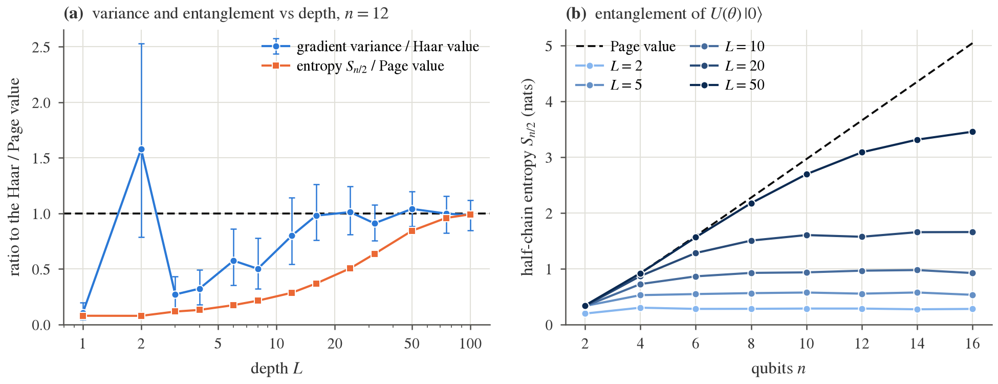
Entanglement-induced plateaus [3] suggest looking at the two quantities together. Figure 2(a) shows, at , that the variance is statistically indistinguishable from the Haar value from – onwards (ratios , , , , at ), whereas the half-chain entropy at is only nats, 37% of the Page value, and reaches 96% of it only at (99% at , where the variance ratio is ). Panel (b) shows the same across : at the entropy is far from Page for every while the variance already decays as . The gradient of a global cost thus sees “enough” randomness much earlier than the bipartite entanglement does; the second moment of the ensemble converges faster than its Page-curve statistics. Conversely, large entanglement is not needed for a plateau in this cost.
5.3 E2: cost-function dependence
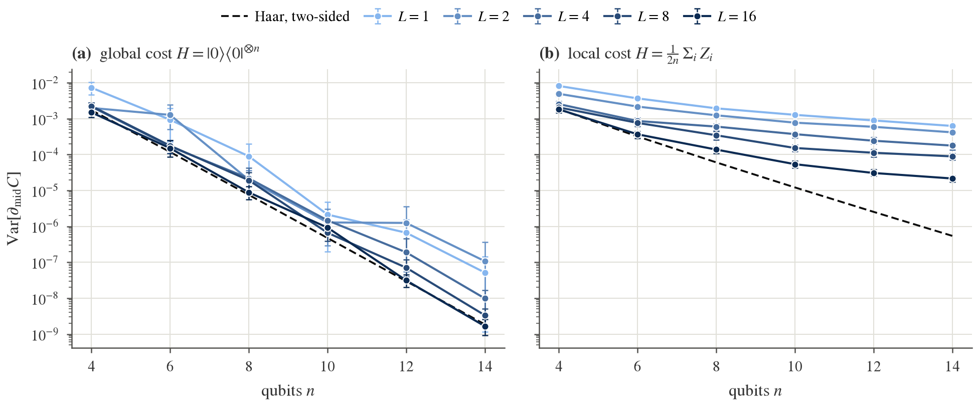
Figure 3 reproduces the central result of [2]. For the projector cost the fitted exponents are to (approaching the Haar scaling with depth), and already at the variance is at . For the local cost the exponents are to : the decay is far slower than at all depths studied and the variance at , is , four orders of magnitude above the global cost at the same size. The local-cost variance also lies well above its own Haar value (dashed) at every depth, i.e. these brick circuits are far from 2-designs for a local observable even at ; the slow drift of the local exponent with is consistent with the -depth window of [2].
5.4 E3: initialisation strategies
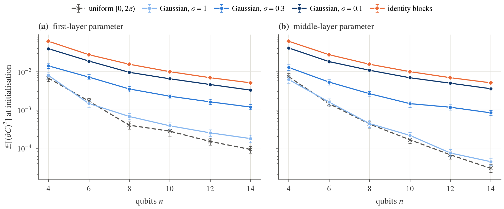
We report the mean square rather than the variance because the identity-block initialisation gives a deterministic first-layer derivative: with every block equal to the identity, for a gate in the first half-layer, so exactly for every random draw (variance zero, magnitude ). Figure 4 shows that small-angle initialisations help as advertised [5]: at the mean-square first-layer derivative is for uniform angles, for and for , with fitted exponents (uniform), (), () and (). The identity-block curve decays as by construction. Two caveats: with this local cost and even the uniform initialisation decays with an exponent well above (cf. Sec. 5.3), and a large gradient at says nothing about the landscape a few steps later, which is the regime that matters [9].
5.5 E5: plateaus versus optimisation
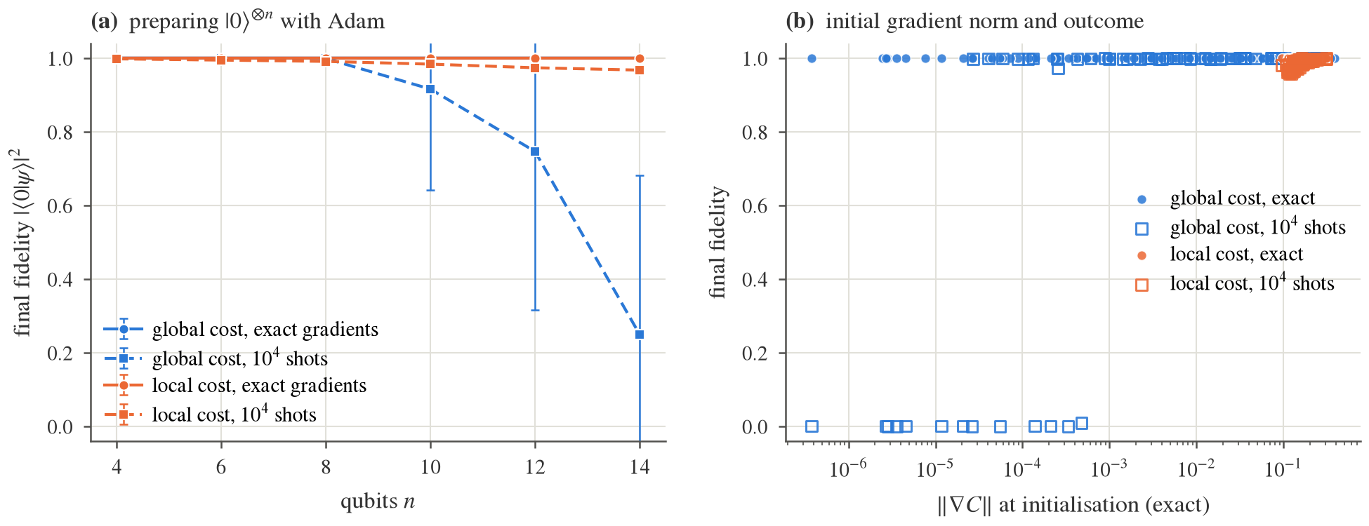
| 4 | 6 | 8 | 10 | 12 | 14 | |
|---|---|---|---|---|---|---|
| global cost, exact gradients | ||||||
| mean fidelity | 1.000 | 1.000 | 1.000 | 1.000 | 1.000 | 1.000 |
| fraction with | 1.00 | 1.00 | 1.00 | 1.00 | 1.00 | 1.00 |
| mean at initialisation | 0.16 | 0.046 | 0.028 | 0.0045 | 0.0022 | 0.00015 |
| local cost, exact gradients | ||||||
| mean fidelity | 1.000 | 1.000 | 1.000 | 1.000 | 1.000 | 1.000 |
| fraction with | 1.00 | 1.00 | 1.00 | 1.00 | 1.00 | 1.00 |
| mean at initialisation | 0.24 | 0.19 | 0.16 | 0.14 | 0.13 | 0.12 |
| global cost, shots | ||||||
| mean fidelity | 0.999 | 0.999 | 0.999 | 0.916 | 0.746 | 0.250 |
| fraction with | 1.00 | 1.00 | 1.00 | 0.92 | 0.75 | 0.25 |
| local cost, shots | ||||||
| mean fidelity | 0.998 | 0.994 | 0.991 | 0.984 | 0.974 | 0.967 |
| fraction with | 1.00 | 1.00 | 1.00 | 1.00 | 1.00 | 1.00 |
A plateau at initialisation does not by itself prevent a classical simulation from training. With exact gradients, Adam — whose update is approximately scale-invariant — reaches fidelity for both costs at every , including the global cost at where the initial gradient norm is (Table 3, Fig. 5). The plateau becomes an obstacle when gradients must be estimated: adding Gaussian noise equivalent to shots per expectation value, the global-cost optimisation degrades from mean fidelity () to (), () and (), while the local cost stays at – with every run above . Panel (b) makes the mechanism explicit: failures occur exactly for the runs whose exact initial gradient norm lies below the noise level . In other words, the operational content of a barren plateau is the exponential number of measurements needed to resolve the gradient, not an intrinsic failure of gradient descent.
5.6 E6: a problem-inspired ansatz — QAOA for MaxCut
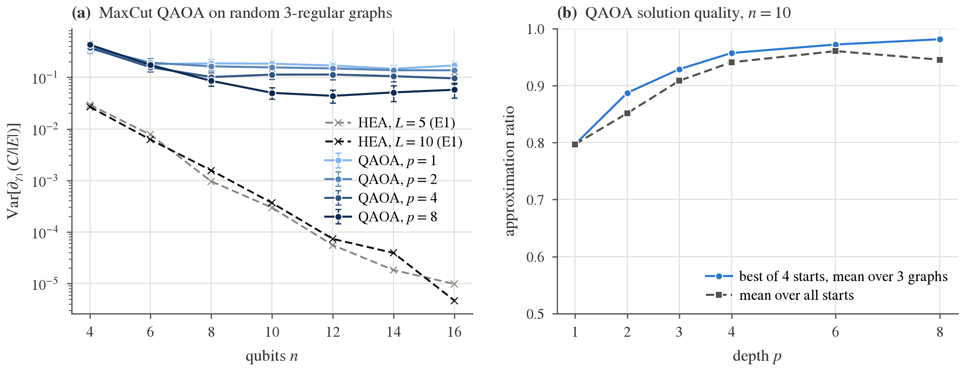
For the HEA the normalised variance decays with exponent ; for QAOA at fixed depth the fitted exponents are (), ( and ) and (): no plateau at fixed depth, consistent with the parameter-concentration results for QAOA and with its small DLA (Sec. 5.7). The price is expressivity: the approximation ratio at grows from at to at and at (best of four starts; the mean over starts saturates at because local optima appear at ).
5.7 E7: dynamical Lie algebras
| family / | 2 | 3 | 4 | 5 | 6 | 7 | 8 | 9 | 10 |
|---|---|---|---|---|---|---|---|---|---|
| DLA dimension | |||||||||
| 15 | 63 | 255 | 1023 | 4095 | 16383 | 65535 | 262143 | 1048575 | |
| HEA | 15 | 63 | 255 | 1023 | 4095 | 16383 | – | – | – |
| HEA | 6 | 15 | 28 | 45 | 66 | 91 | 120 | – | – |
| QAOA MaxCut | – | – | 15 | – | 176 | – | – | – | – |
| HVA TFIM | 4 | 9 | 16 | 25 | 36 | 49 | 64 | 81 | 100 |
| measured / predicted | |||||||||
| HEA | 1.09 | 0.94 | 1.04 | 0.96 | 1.11 | 0.89 | – | – | – |
| HEA | 1.00 | 1.08 | 1.02 | 1.03 | 1.06 | 0.94 | 0.98 | – | – |
| QAOA MaxCut | – | – | 0.60 | – | 0.59 | – | – | – | – |
| HVA TFIM | 0.32 | 1.22 | 0.86 | 1.00 | 1.00 | 1.03 | 0.91 | 1.03 | 0.94 |
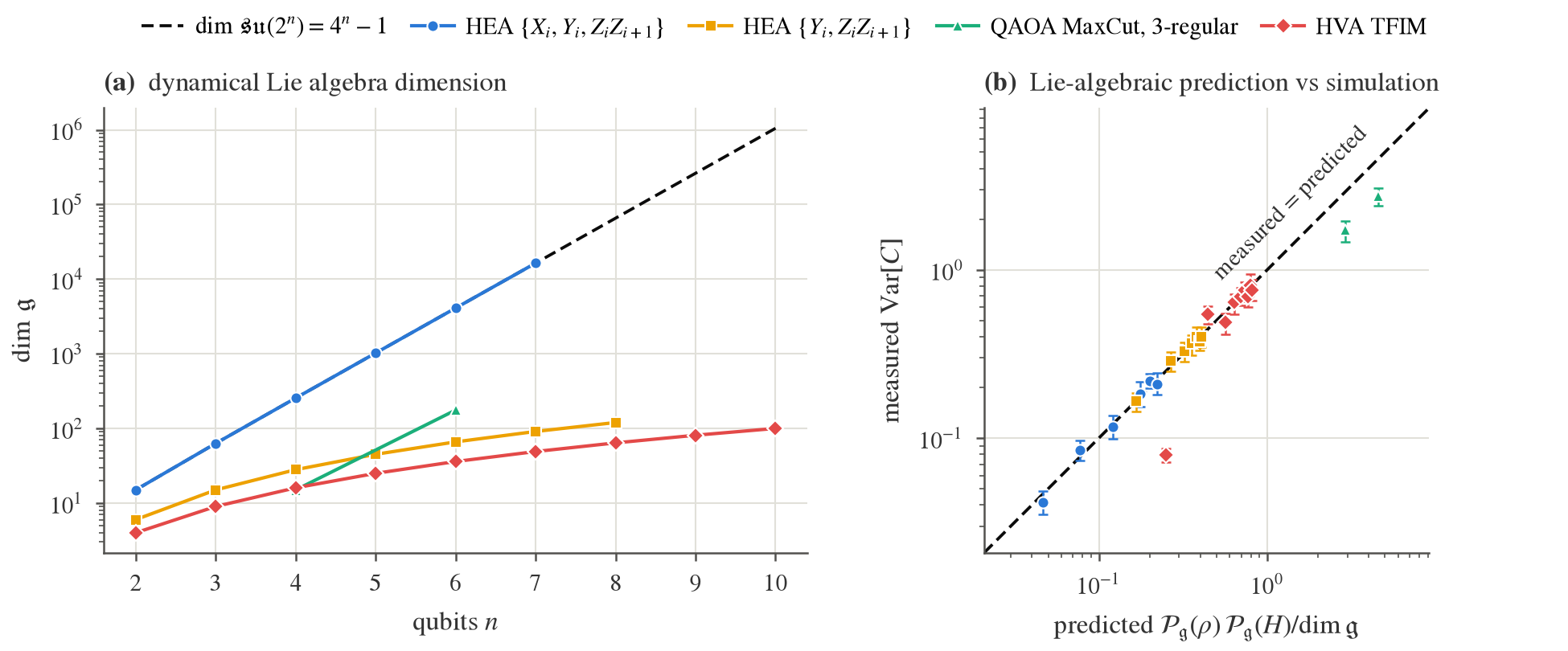
We consider four families whose gates are all Pauli rotations with their own parameters unless stated: (a) (an HEA with and layers); (b) (the same without ); (c) the Hamiltonian variational ansatz of the transverse-field Ising chain, with two shared parameters per layer; (d) QAOA for MaxCut on a random 3-regular graph, . The cost is (the cut operator for (d)), which is an element of in every case, and the initial state is ( for (d)). DLAs are computed exactly: when every generator is a single Pauli string the closure is a breadth-first search over strings (commutators of Pauli strings are Pauli strings); otherwise we run an incremental Gram–Schmidt closure in the Pauli basis. The -purities and follow from the resulting orthonormal basis.
The results (Fig. 7, Table 4) show two polynomial and two exponential families. Family (a) generates the full at every tested, and family (d) grows quickly ( at , at ). Family (b), despite looking like a generic hardware-efficient ansatz, has : it is , the algebra of quadratic forms in Majorana operators — under a Jordan–Wigner transformation and are quadratic in fermions, so this circuit is a free-fermion (matchgate-like) circuit [13]. Family (c), with only two global generators, closes into an even smaller -dimensional subalgebra. Equation (3) is quantitatively accurate for (a), (b) and (c): the ratio of measured to predicted variance is –, – and – respectively (for ; median over all points ). The only clear failures are the smallest TFIM instance (, ratio ) and QAOA (ratios and ), where a circuit with two parameters per layer evidently does not form a 2-design on at , which is the assumption behind Eq. (3).
The polynomial algebra of family (b) has a direct consequence for trainability: for a cost in , is rather than , and indeed the measured variances in Table 4 increase with for (b) and (c) (because grows faster than ). This does not contradict E1–E3, which use costs outside the algebra or ansätze with rotations: adding a single rotation family () turns into .
6 Discussion and limitations
What the numerics add to the theory.
The exact Haar values of Appendix A let us quantify how far a given finite-depth circuit is from the asymptotic regime instead of only checking the exponent. Doing so exposed the undershoot at intermediate depth, the heavy tails that make shallow-depth variance estimates unreliable (and that are a cheap diagnostic of the 2-design regime), and the decoupling between the convergence of the gradient variance and of the entanglement entropy. The DLA study turned a seemingly generic hardware-efficient family into a free-fermion circuit with a polynomial algebra, and confirmed Eq. (3) with exact purities rather than estimates.
Limitations.
All simulations are noiseless apart from the Gaussian shot-noise model of E5; noise-induced plateaus are a separate phenomenon. We go to at most 16 qubits, so exponents are fitted over about a decade of ; the heavy tails at shallow depth widen the intervals of the smallest-depth points, and the points at use only 100 samples. E5 uses a single optimiser configuration and a small learning-rate/step budget; the shot-noise model is additive Gaussian rather than binomial. For QAOA, the graph is resampled with the parameters, so the variance mixes graph and parameter randomness. The DLA closure caps at a few thousand dimensions, which limits QAOA to . Finally, the report is a reproduction-and-consolidation study: its new observations are empirical and would need larger and more ensembles to become claims.
7 Conclusion
A few hundred lines of NumPy, exact gradients and a few CPU-hours are enough to test the barren-plateau literature quantitatively rather than qualitatively. The main predictions — decay for 2-design circuits, versus slow decay for global versus local costs, the benefit of small-angle initialisation, the absence of plateaus at fixed QAOA depth, and the Lie-algebraic variance formula — all hold within the stated accuracies. Along the way we found that the approach to the plateau is non-monotonic and heavy-tailed, that it precedes the saturation of entanglement, that exact-gradient optimisation is blind to the plateau at these sizes while finite-shot optimisation is not, and that a common hardware-efficient family is secretly free-fermionic. The code, data and a single make target to regenerate every figure are released with this report.
Code and data availability
The simulator, the ansatz and experiment scripts, the cached results for every data point and the scripts that regenerate every figure and table are available at https://github.com/thanatchon36/bp-from-scratch under the MIT licence and archived on Zenodo (doi:10.5281/zenodo.23995488, version 0.2.0). The results are also published as a dataset at https://huggingface.co/datasets/thanatchon36/bp-from-scratch; Appendix C lists the commands.
A Haar averages of the gradient variance
Write the circuit around a rotation with Pauli generator (, ) as , let and with . Since and , with and Hermitian and traceless. We use the standard second moments of a Haar-random pure state in dimension , , and of a Haar-random unitary,
Random circuit after the rotation only ().
Then is fixed, is fixed, and is a Haar conjugate of . With and for a pure ,
Random circuit before the rotation only ().
Then and is a Haar-random pure state. With , and , For and an or rotation on one qubit, and the variance is ; for a rotation it vanishes. Averaging over the random axes of the McClean ensemble gives for the last-layer probe of Sec. 5.1.
Random circuits on both sides.
Averaging Eq. (8) over the Haar conjugate of (independent of ) with the four-fold formula gives and hence which is Eq. (2): for a traceless Pauli string and for the projector . Table 5 compares the three formulas with direct sampling of Haar unitaries (400 samples, on qubit 0, uniform).
| two-sided | after only () | before only () | ||||
| simulated | Eq. (2) | simulated | Eq. (7) | simulated | Eq. (8) | |
| 2 | ||||||
| 3 | ||||||
| 4 | ||||||
| 5 | ||||||
| 6 | ||||||
| 7 | ||||||
| 8 | ||||||
| 2 | ||||||
| 3 | ||||||
| 4 | ||||||
| 5 | ||||||
| 6 | ||||||
| 7 | ||||||
| 8 | ||||||
B Adjoint-mode gradient
Let and . For a rotation , and therefore Sweeping from down to while applying to both and computes every term with three state-vector operations per gate and no extra memory [10]; shared parameters accumulate automatically. The parameter-shift rule, Eq. (1), is applied to one gate occurrence at a time and summed; both agree with finite differences to in the test suite.
C Reproduction
pip install -e ".[dev]"              # or ".[dev,compare]" for PennyLane checks
python -m pytest -q                  # 58 tests
BUDGET=100000 bash experiments/run_all.sh   # all experiments, ~1 CPU hour
python analysis/make_figures.py      # paper/figures/*.pdf, results/figures/*.png
python analysis/make_tables.py       # paper/tables/*.tex
bash paper/build.sh                  # PDF, web reader, Markdown mirror
Every experiment script skips cached points, so an interrupted run resumes where it stopped. Figures and tables in this document were produced by exactly these commands from the committed results/ directory.
References
J. R. McClean, S. Boixo, V. N. Smelyanskiy, R. Babbush, H. Neven, Barren plateaus in quantum neural network training landscapes, Nat. Commun. 9, 4812 (2018), doi:10.1038/s41467-018-07090-4.
M. Cerezo, A. Sone, T. Volkoff, L. Cincio, P. J. Coles, Cost function dependent barren plateaus in shallow parametrized quantum circuits, Nat. Commun. 12, 1791 (2021), doi:10.1038/s41467-021-21728-w.
C. Ortiz Marrero, M. Kieferová, N. Wiebe, Entanglement-induced barren plateaus, PRX Quantum 2, 040316 (2021), doi:10.1103/PRXQuantum.2.040316.
E. Grant, L. Wossnig, M. Ostaszewski, M. Benedetti, An initialization strategy for addressing barren plateaus in parametrized quantum circuits, Quantum 3, 214 (2019), doi:10.22331/q-2019-12-09-214.
K. Zhang, L. Liu, M.-H. Hsieh, D. Tao, Escaping from the barren plateau via Gaussian initializations in deep variational quantum circuits, Adv. Neural Inf. Process. Syst. 35, 18612–18627 (2022), arXiv:2203.09376.
M. Larocca, P. Czarnik, K. Sharma, G. Muraleedharan, P. J. Coles, M. Cerezo, Diagnosing barren plateaus with tools from quantum optimal control, Quantum 6, 824 (2022), doi:10.22331/q-2022-09-29-824.
M. Ragone, B. N. Bakalov, F. Sauvage, A. F. Kemper, C. Ortiz Marrero, M. Larocca, M. Cerezo, A Lie algebraic theory of barren plateaus for deep parameterized quantum circuits, Nat. Commun. 15, 7172 (2024), doi:10.1038/s41467-024-49909-3.
E. Fontana, D. Herman, S. Chakrabarti, N. Kumar, R. Yalovetzky, J. Heredge, S. H. Sureshbabu, M. Pistoia, Characterizing barren plateaus in quantum ansätze with the adjoint representation, Nat. Commun. 15, 7171 (2024), doi:10.1038/s41467-024-49910-w.
M. Larocca, S. Thanasilp, S. Wang, K. Sharma, J. Biamonte, P. J. Coles, L. Cincio, J. R. McClean, Z. Holmes, M. Cerezo, Barren plateaus in variational quantum computing, Nat. Rev. Phys. 7, 174–189 (2025), doi:10.1038/s42254-025-00813-9.
T. Jones, J. Gacon, Efficient calculation of gradients in classical simulations of variational quantum algorithms, arXiv:2009.02823 (2020).
D. N. Page, Average entropy of a subsystem, Phys. Rev. Lett. 71, 1291–1294 (1993), doi:10.1103/PhysRevLett.71.1291.
E. Farhi, J. Goldstone, S. Gutmann, A quantum approximate optimization algorithm, arXiv:1411.4028 (2014).
E. Kökcü, T. Steckmann, Y. Wang, J. K. Freericks, E. F. Dumitrescu, A. F. Kemper, Fixed depth Hamiltonian simulation via Cartan decomposition, Phys. Rev. Lett. 129, 070501 (2022), doi:10.1103/PhysRevLett.129.070501.